NALgen Analysis Pt.1 - Recap
The output of multivariate analyses in the NALgen Analysis Pt.1 post was dense (935 lines of code, 121 figures). In this recap, I wanted to highlight some of the results. Furthermore, I wanted to mention that the population structure inference methods I compared were all machine learning (classification) algorithms.
DAPC is an unsupervised-supervised learning algorithm (principal components analysis = unsupervised, discriminant analysis = supervised). Non-negative matrix factorization algorithms implemented in the LEA and tess3r packages are both cases of unsupervised machine learning; both use least-squares estimates of ancestry coefficients, which are geographically constrained in tess3r (i.e., spatial/geographic weights are used).
All three methods are rather fast and produced similar results.
- DAPC went through 24 data sets in 17 mins,
- LEA processed 8 in 38 mins (however, it should be noted that this included 5 replicates x 15 values of K = 75),
- tess3r processed 8 in 122 mins (also 5 replicates x 15 values of K).
The NALgen method leverages the flexibility of the co-inertia method (N.B. other multivariate ordination techniques can be used) to incorporate genetic clustering (i.e., population structure) information from any algorithm (see the co-inertia section below). The idea behind this is to first determine the variance in genetic data explained by processes that have led to the inferred population structure, and then identify covariance with environmental data. This information can then be used downstream in the NALgen method (modeling gene flow in continuous space).
Color palette
library(ggsci)
library(scales)

futr <- pal_futurama()
schwifty <- pal_rickandmorty()
futr.cols <- colorRampPalette(futr(12)[c(12,11,3,7,8,6,1,2)])
schwifty.cols <- colorRampPalette(schwifty(12)[c(3,12,4,6,1,9,8,2)])
futrschwift.cols <- colorRampPalette(c("gray15", schwifty(12)[3], futr(12)[11], schwifty(12)[c(1,9)], futr(12)[c(8,6,2)]))
cols <- futrschwift.cols(12)

#show_col(futr.cols(20))
#show_col(schwifty.cols(20))
#show_col(futrschwift.cols(20))
Multivariate analyses: Using machine learning algorithms to infer population structure
Loading the environmental data
library(raster)
library(virtualspecies)

setwd("C:/Users/chazh/Documents/Research Projects/Reticulitermes/Phylogeography/Geo_Analysis/Data/EnvData/bioclim_FA/east coast/Finalized/current")
fn <- list.files(pattern=".asc")
fa_stk <- stack()
for(i in 1:length(fn)) fa_stk=addLayer(fa_stk,raster(fn[i]))

#names for plot titles
fa_stk_names <- c("Annual Temperature Range", "Dry-Season Precipitation", "Summer Temperature", "Wet-Season Precipitation")

##plot Environmental Factors (https://datadryad.org/resource/doi:10.5061/dryad.5hr7f31)
#for (i in 1:4){
#   plot(fa_stk[[i]], main=fa_stk_names[i],
#       breaks=seq(round(min(as.matrix(fa_stk[[i]]),na.rm=T),1),
#                  round(max(as.matrix(fa_stk[[i]]),na.rm=T),1),length.out=11),
#       col=cols)
#}
Loading the genetic data (only 2, vs. 24 in the NALgen Analysis Pt.1 post)
library(adegenet)


m0.5_n.s <- "C:/Users/chazh/Documents/Research Projects/Reticulitermes/Simulations/popRange/m_0_5/Simulated_Genotypes/20pop_subsets/neutral+selected/"


setwd("C:/Users/chazh/Documents/Research Projects/Reticulitermes/NALgen_Analysis/Multivariate/")

#below I define the xyFromRC function: includes a scenario when genind and rastr don't have the same dimensions
#currently (for my purposes here it's fine) only spits out error when aspect ratio is not the same, but proceeds the same anyway
#need to fix to apply to other situations

xyFromRC <- function(genind, rastr){
             coord <- genind$other
             row.no <- coord[,1]+1
             col.no <- coord[,2]+1
             dim.genind.row <- 26 #dim of simulated landscape
             dim.genind.col <- 34 #dim of simulated landscape
             dim.rast.row <- dim(rastr)[1]
             dim.rast.col <- dim(rastr)[2]
             if(dim.rast.col/dim.genind.col == dim.rast.row/dim.genind.row){
                print("raster and genind are the same aspect ratio. proceed.")
             }
             else{
                print("error! raster and genind are NOT the same aspect ratio. proceed ANYWAY.")
             }
             rastr <- aggregate(rastr, dim.rast.col/dim.genind.col)
             cell.no <- cellFromRowCol(rastr, row=row.no, col=col.no)
             coord <- xyFromCell(rastr, cell.no)
             as.data.frame(coord)
         }

#use already aggregated fa_stk to make this go faster
fa_stk.agg <- aggregate(fa_stk, dim(fa_stk)[1]/26)

###m0.5###
##neutral AND selected##
m0.5_hchp_n.s <- read.genepop(paste0(m0.5_n.s,"hchp_20pops.gen"))
m0.5_hchp_n.s$other <- read.table(paste0(m0.5_n.s,"hchp_20pops_coords.txt"), sep=" ",header=F)
colnames(m0.5_hchp_n.s$other)=c("x","y")
m0.5_hchp_n.s$other <- xyFromRC(m0.5_hchp_n.s, fa_stk.agg)
m0.5_hclp_n.s <- read.genepop(paste0(m0.5_n.s,"hclp_20pops.gen"))
m0.5_hclp_n.s$other <- read.table(paste0(m0.5_n.s,"hclp_20pops_coords.txt"), sep=" ",header=F)
colnames(m0.5_hclp_n.s$other)=c("x","y")
m0.5_hclp_n.s$other <- xyFromRC(m0.5_hclp_n.s, fa_stk.agg)
Co-Inertia Analysis: Genetic-environmental covariance
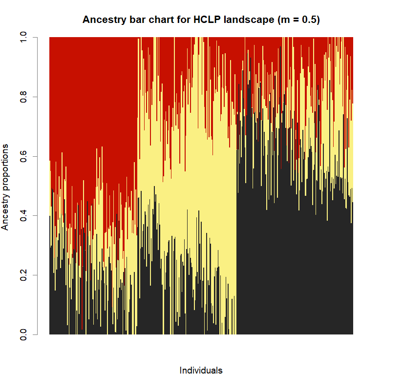
Co-Inertia Analysis is used to determine the maximum covariance between genetic and environmental data at the spatial scale at which populations become differentiated (population structuring). To do so, population structure is first inferred (classification into genetic clusters) using unsupervised (and unsupervised-supervised) machine learning methods.
Unsupervised classification: Inferring genetic clusters using non-negative matrix factorization (LEA package)
High-complexity landscapes (m = 0.5)
library(LEA)
library(mapplots)
library(maps)
futr <- pal_futurama()
schwifty <- pal_rickandmorty()
futrschwift.cols <- colorRampPalette(c("gray15", schwifty(12)[3], futr(12)[11], schwifty(12)[c(1,9)], futr(12)[c(8,6,2)]))
#plot parameters
par(mfrow=c(1,1),fg="gray50",pty='m',bty='o',mar=c(4,4,4,4),cex.main=1.3,cex.axis=1.1,cex.lab=1.2)
geninds <- list(m0.5_hclp_n.s,
m0.5_hchp_n.s)
genind_names <- c("m0.5_hclp_n.s",
"m0.5_hchp_n.s")
ls_names <- c("HCLP landscape (m = 0.5)",
"HCHP landscape (m = 0.5)")
lea.dir <- c(
"C:/Users/chazh/Documents/Research Projects/Reticulitermes/Simulations/popRange/m_0_5/Simulated_Landscapes/500neutral+50selectedSNPs/High_Complexity_Landscapes/virtualspecies/Low_Permeability/",
"C:/Users/chazh/Documents/Research Projects/Reticulitermes/Simulations/popRange/m_0_5/Simulated_Landscapes/500neutral+50selectedSNPs/High_Complexity_Landscapes/virtualspecies/High_Permeability/"
)
for (i in 1:2){
genind.obj <- geninds[[i]]
genotypes <- genind.obj$tab
coords <- genind.obj$other
setwd(lea.dir[i])
write.table(t(as.matrix(genotypes)), sep="", row.names=F, col.names=F, paste0(genind_names[i], ".geno"))
geno <- read.geno(paste0(genind_names[i],".geno"))
setwd(paste0(lea.dir[i],"LEA"))
source("POPSutilities.r")
setwd(lea.dir[i])
reps <- 5
maxK <- 15
#running pop structure inference
snmf.obj <- snmf(paste0(genind_names[i],".geno"), K=1:maxK, repetitions=reps, project="new",
alpha=10, iterations=100000,
entropy=TRUE, percentage=0.25)
plot(snmf.obj, cex=1.2, col="lightblue", pch=19)
#determining best K and picking best replicate for best K
ce <- list()
for(k in 1:maxK) ce[[k]] <- cross.entropy(snmf.obj, K=k)
best <- which.min(unlist(ce))
best.K <- ceiling(best/reps)
best.run <- which.min(ce[[best.K]])
barchart(snmf.obj, K=best.K, run=best.run,
border=NA, space=0, col=futrschwift.cols(best.K),
xlab="Individuals", ylab="Ancestry proportions",
main=paste("Ancestry bar chart for", ls_names[i]))
qmatrix <- Q(snmf.obj, K=best.K, run=best.run)
grid <- createGrid(xmin(fa_stk), xmax(fa_stk),
ymin(fa_stk), ymax(fa_stk), 260, 340)
constraints <- NULL
shades <- 10
futrschwift.gradient <- colorRampPalette(futrschwift.cols(best.K))
grad.cols <- futrschwift.gradient(shades*best.K)
ColorGradients_bestK <- list()
for(j in 1:best.K){
k.start <- j*shades-shades+1
k.fin <- j*shades
ColorGradients_bestK[[j]] <- c("gray95", grad.cols[k.start:k.fin])
}
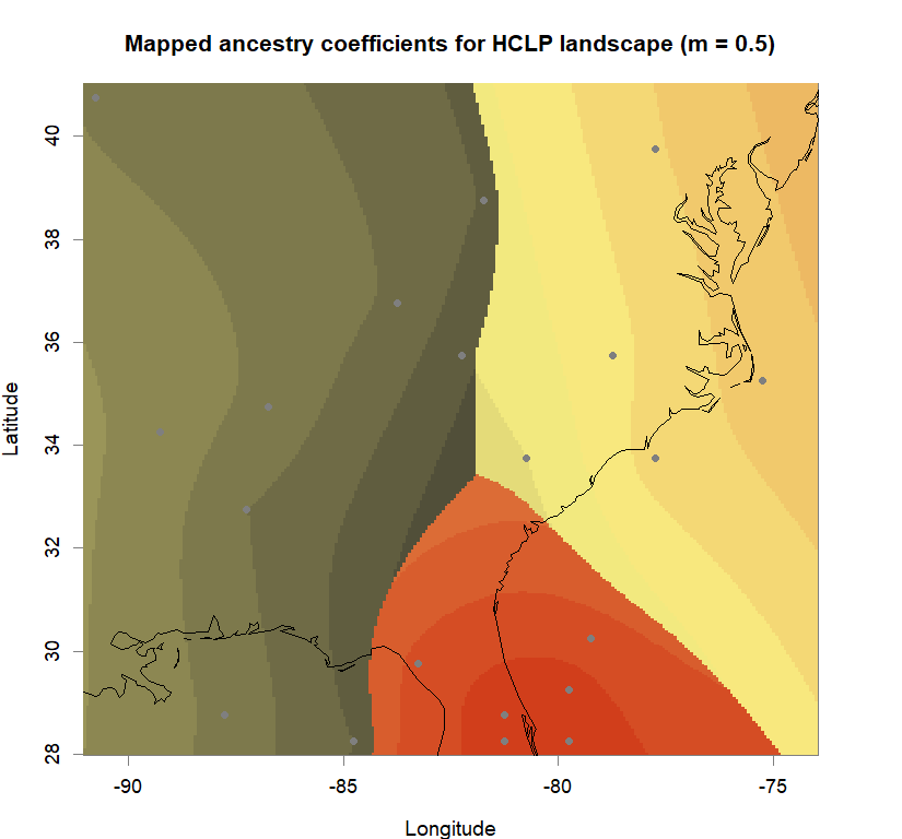
maps(qmatrix, coords, grid, constraints, method="max",
colorGradientsList=ColorGradients_bestK,
main=paste("Mapped ancestry coefficients for", ls_names[i]),
xlab="Longitude", ylab="Latitude", cex=.5)
map(add=T, interior=F)
}


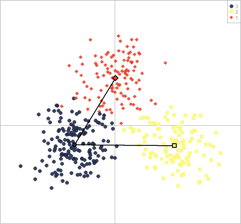
Unsupervised-supervised classification: Inferring genetic clusters using DAPC
High-complexity landscapes (m = 0.5): low permeability
#genetic data
gen <- m0.5_hclp_n.s
Setting up the data (genetic and environmental)
dfenv <- extract(fa_stk, gen$other)
dfenv.obj <- dfenv
dfgen.obj <- gen$tab
dfgenenv <- cbind(dfgen.obj, dfenv.obj)
dfgenenv <- na.omit(dfgenenv)
n.alleles <- length(dfgen.obj[1,])
n.env <- length(dfenv.obj[1,])
env.var <- seq(n.alleles + 1, n.alleles + n.env)
dfgen <- dfgenenv[,1:n.alleles]
dfenv <- dfgenenv[,env.var]
Running DAPC
#plot parameters
par(mfrow=c(1,1), fg="gray50", pty='m', bty='o', mar=c(4,4,4,4), cex.main=1.3, cex.axis=1.1, cex.lab=1.2)
cols3 <- futrschwift.cols(12)[c(2,6,11)]

temp.dapc.obj <- dapc(gen, center=T, scale=F, n.pca=100, n.da=2)
temp <- optim.a.score(temp.dapc.obj, n=15, n.sim=30)

best.n.pca <- temp$best
dapc.obj <- dapc(gen, center=T, scale=F, n.pca=best.n.pca, n.da=2)
clust <- find.clusters(gen, cent=T, scale=F, n.pca=best.n.pca, method="kmeans", n.iter=1e7, n.clust=3, stat="BIC")
cl <- as.factor(as.vector(clust$grp))
gen$pop <- cl
sq <- as.character(seq(1,3))
popNames(gen) <- sq
dapc3 <- dapc(gen, center=T, scale=F, n.pca=best.n.pca, n.da=2)
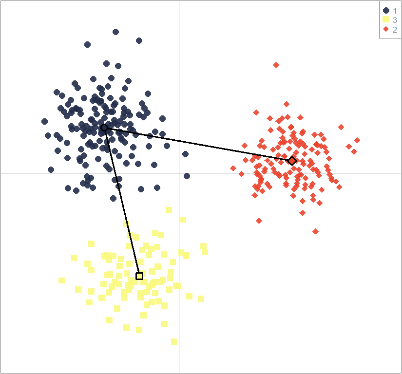
scatter(dapc3, col=cols3, ratio.pca=0.3, bg="white",
pch=c(16,15,18,17), cell=0, cstar=0, solid=0.9, cex=1.8, clab=0,
mstree=TRUE, lwd=3, scree.da=FALSE, leg=TRUE, txt.leg=popNames(gen))
par(xpd=TRUE)
points(dapc3$grp.coord[,1], dapc3$grp.coord[,2], pch=21:24, cex=2, lwd=3, col="black", bg=cols3)
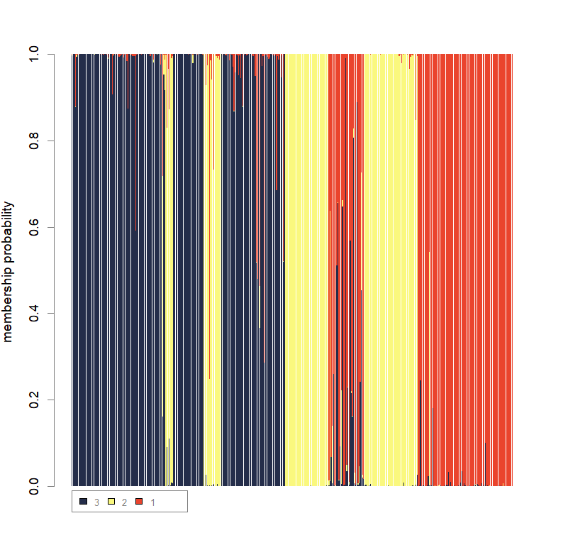
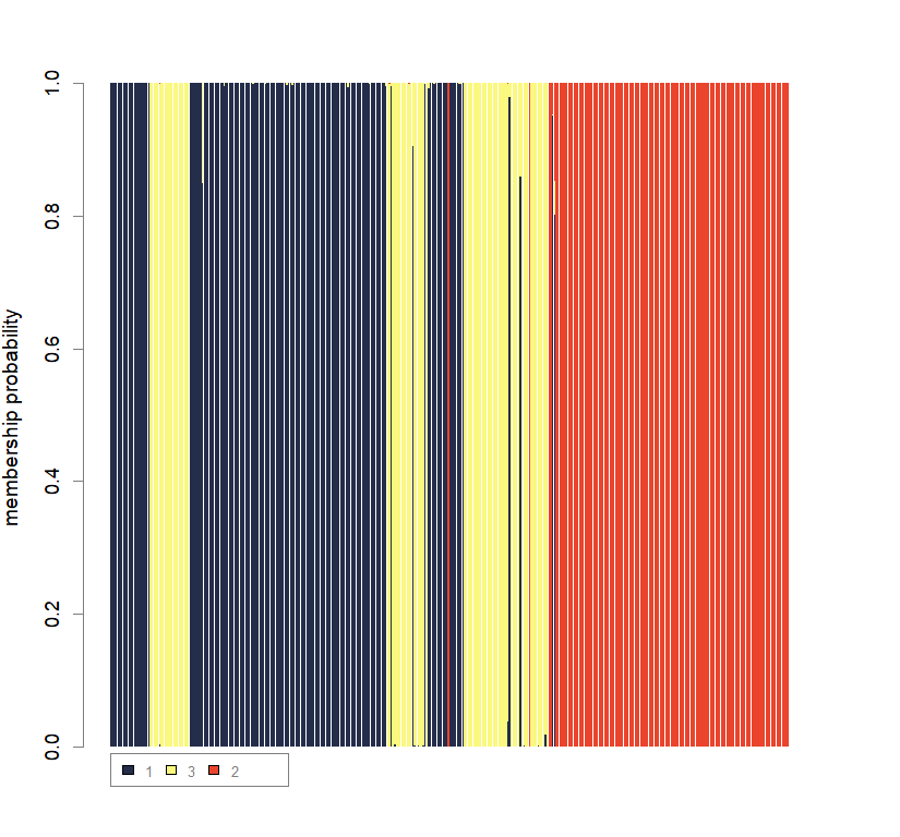
compoplot(dapc3, lab="", col=cols3)
dap3 <- as.data.frame(dapc3$assign)
dfdap3 <- cbind(dap3, dfenv.obj)
dfdap3 <- na.omit(dfdap3)
dfenv3 <- dfdap3[,2:length(dfdap3[1,])]
dfdap3 <- dfdap3[,1]

dfgenenv3 <- cbind(dap3, dfgen.obj, dfenv.obj)
dfgenenv3 <- na.omit(dfgenenv3)
dfdap3 <- dfgenenv3[,1]
dfgenenv3.gen <- dfgenenv3[,2:n.alleles+1]
dfgenenv3.env <- dfgenenv3[,env.var+1]
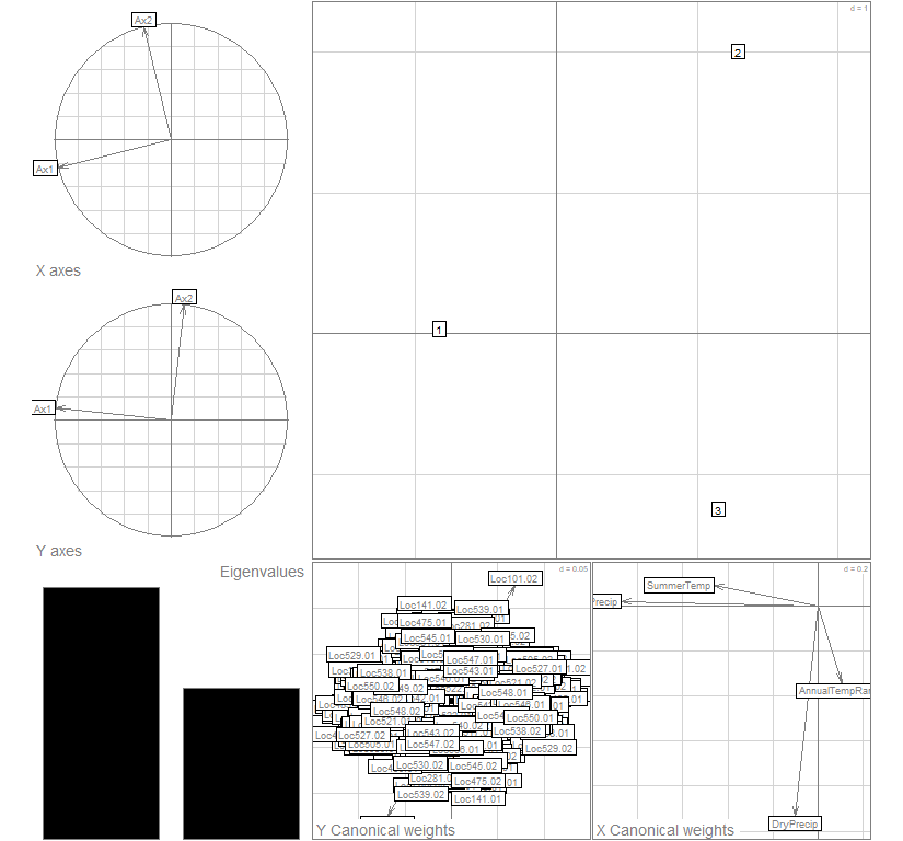
Co-Inertia Analysis: Maximizing genetic-environmental covariance (using inferred genetic clusters as constraint)
The DAPC classification (of locations/individuals into one of three inferred genetic clusters) is used as a constraint (constrained correspondence analysis) to determine the variance in genetic data explained by processes that have led to the inferred population structure, and Co-Inertia Analysis is then used to look at covariance with environmental data.
pcenv3 <- dudi.pca(dfenv3, cent=T, scale=T, scannf=F, nf=2)

#dfdap3 = DAPC classification

#constrained correspondence analysis of environmental data
bet1 <- bca(pcenv3, dfdap3, scannf=F, nf=2)

pcgen3 <- dudi.pca(dfgen, cent=T, scale=F, scannf=F, nf=2)

#constrained correspondence analysis of genetic data
bet2 <- bca(pcgen3, dfdap3, scannf=F, nf=2)

#maximizing genetic-environmental covariance (at the scale of three populations)
coi3 <- coinertia(bet1, bet2, scan=F, nf=2)

par(mfrow=c(1,1), fg="gray50", pty='m', bty='o', mar=c(4,4,4,4), cex.main=1.3, cex.axis=1.1, cex.lab=1.2)

plot(coi3, col="gray30")

summary(coi3)
## Coinertia analysis
##
## Class: coinertia dudi
## Call: coinertia(dudiX = bet1, dudiY = bet2, scannf = F, nf = 2)
##
## Total inertia: 17.69
##
## Eigenvalues:
##     Ax1     Ax2
##  15.708   1.984
##
## Projected inertia (%):
##     Ax1     Ax2
##   88.79   11.21
##
## Cumulative projected inertia (%):
##     Ax1   Ax1:2
##   88.79  100.00
##
## Eigenvalues decomposition:
##         eig    covar       sdX      sdY      corr
## 1 15.708356 3.963377 1.3465110 2.948251 0.9983689
## 2  1.983529 1.408378 0.5264643 2.679534 0.9983689
##
## Inertia & coinertia X (bet1):
##     inertia      max     ratio
## 1  1.813092 1.814158 0.9994126
## 12 2.090256 2.090256 1.0000000
##
## Inertia & coinertia Y (bet2):
##      inertia       max     ratio
## 1   8.692183  8.816482 0.9859015
## 12 15.872087 15.872087 1.0000000
##
## RV:
##  0.8537908
Another iteration (with a different landscape)
High-complexity landscapes (m = 0.5): high permeability
#genetic data
gen <- m0.5_hchp_n.s
Setting up the data (genetic and environmental)
dfenv <- extract(fa_stk, gen$other)
dfenv.obj <- dfenv
dfgen.obj <- gen$tab
dfgenenv <- cbind(dfgen.obj, dfenv.obj)
dfgenenv <- na.omit(dfgenenv)
n.alleles <- length(dfgen.obj[1,])
n.env <- length(dfenv.obj[1,])
env.var <- seq(n.alleles + 1, n.alleles + n.env)
dfgen <- dfgenenv[,1:n.alleles]
dfenv <- dfgenenv[,env.var]
Running DAPC
#plot parameters
par(mfrow=c(1,1), fg="gray50", pty='m', bty='o', mar=c(4,4,4,4), cex.main=1.3, cex.axis=1.1, cex.lab=1.2)

temp.dapc.obj <- dapc(gen, center=T, scale=F, n.pca=100, n.da=2)
temp <- optim.a.score(temp.dapc.obj, n=15, n.sim=30)

best.n.pca <- temp$best
dapc.obj <- dapc(gen, center=T, scale=F, n.pca=best.n.pca, n.da=2)
clust <- find.clusters(gen, cent=T, scale=F, n.pca=best.n.pca, method="kmeans", n.iter=1e7, n.clust=3, stat="BIC")
cl <- as.factor(as.vector(clust$grp))
gen$pop <- cl
sq <- as.character(seq(1,3))
popNames(gen) <- sq

dapc3 <- dapc(gen, center=T, scale=F, n.pca=best.n.pca, n.da=2)
scatter(dapc3, col=cols3, ratio.pca=0.3, bg="white",
    pch=c(16,15,18,17), cell=0, cstar=0, solid=0.9, cex=1.8, clab=0,
    mstree=TRUE, lwd=3, scree.da=FALSE, leg=TRUE, txt.leg=popNames(gen))
par(xpd=TRUE)
points(dapc3$grp.coord[,1], dapc3$grp.coord[,2], pch=21:24, cex=2, lwd=3, col="black", bg=cols3)
compoplot(dapc3, lab="", col=cols3)
dap3 <- as.data.frame(dapc3$assign)
dfdap3 <- cbind(dap3, dfenv.obj)
dfdap3 <- na.omit(dfdap3)
dfenv3 <- dfdap3[,2:length(dfdap3[1,])]
dfdap3 <- dfdap3[,1]

dfgenenv3 <- cbind(dap3, dfgen.obj, dfenv.obj)
dfgenenv3 <- na.omit(dfgenenv3)
dfdap3 <- dfgenenv3[,1]
dfgenenv3.gen <- dfgenenv3[,2:n.alleles+1]
dfgenenv3.env <- dfgenenv3[,env.var+1]
Co-Inertia Analysis
pcenv3 <- dudi.pca(dfenv3, cent=T, scale=T, scannf=F, nf=2)

#dfdap3 = DAPC classification

#constrained correspondence analysis of environmental data
bet1 <- bca(pcenv3, dfdap3, scannf=F, nf=2)

pcgen3 <- dudi.pca(dfgen, cent=T, scale=F, scannf=F, nf=2)

#constrained correspondence analysis of genetic data
bet2 <- bca(pcgen3, dfdap3, scannf=F, nf=2)

#maximizing genetic-environmental covariance (at the scale of three populations)
coi3 <- coinertia(bet1, bet2, scan=F, nf=2)

par(mfrow=c(1,1), fg="gray50", pty='m', bty='o', mar=c(4,4,4,4), cex.main=1.3, cex.axis=1.1, cex.lab=1.2)

plot(coi3, col="gray30")
summary(coi3)
## Coinertia analysis
##
## Class: coinertia dudi
## Call: coinertia(dudiX = bet1, dudiY = bet2, scannf = F, nf = 2)
##
## Total inertia: 5.563
##
## Eigenvalues:
##     Ax1     Ax2
##   3.481   2.082
##
## Projected inertia (%):
##     Ax1     Ax2
##   62.57   37.43
##
## Cumulative projected inertia (%):
##     Ax1   Ax1:2
##   62.57  100.00
##
## Eigenvalues decomposition:
##        eig    covar       sdX      sdY      corr
## 1 3.480530 1.865618 0.6102563 3.059683 0.9991576
## 2 2.082317 1.443024 0.5640759 2.560365 0.9991576
##
## Inertia & coinertia X (bet1):
##      inertia       max     ratio
## 1  0.3724128 0.3758718 0.9907973
## 12 0.6905944 0.6905944 1.0000000
##
## Inertia & coinertia Y (bet2):
##      inertia       max     ratio
## 1   9.361659  9.398018 0.9961313
## 12 15.917129 15.917129 1.0000000
##
## RV:
##  0.9920957
Final note
To determine the maximum genetic-environmental covariance, the raw data is first transformed. It is these transformed environmental scores that form the predictors in NALgen modeling: the idea here is that these transformed environmental scores are more informative for modeling a genetic response than the raw environmental data. The response variables are measures of genetic variation (neutral and adaptive): these are newly-developed metrics that I will be introducing in upcoming posts.